When astronauts look at the Earth from orbit, they are often awed by its beauty and isolation. They speak of the overview effect; a cognitive shift to a new larger perspective that gives context and meaning to their lives. For physicists, a similar, more abstract overview effect can come from the perusal of log-log plots.

Fig. 1 is our recently published pedagogical plot of all the objects in the universe.  Like the Standard Model, it is an incomplete work in progress. It can help students and physicists articulate some fundamental questions about the incompleteness and limits of physics and the Standard Model.

On the left, the smallest possible object in the universe (an instanton) has the Planck length and Planck mass. In the upper right, the largest possible object in the universe is the universe itself, represented by the mass inside the Hubble radius. Both the instanton and the Hubble radius lie on the black hole line with their Schwarzschild radii proportional to their mass.  This diagonal line of black holes is the boundary of the “forbidden by gravity” region. For a given mass, no object is smaller than a black hole of that mass. For a given size, no object is more massive than a black hole of that size.  In the past, the universe was smaller but it was always on the black hole line. Although suggestive, this does not mean the universe is a black hole unless our universe is surrounded by empty Minkowski space (one of the assumptions made when computing a Schwarzschild radius).

The diagonal Compton limit line (r ~ m^-1) is interestingly orthogonal to the black hole line and extends from the instanton on the far left, down through the particles of the Standard Model (top quark, Higgs, W^±, neutron, proton, electron, neutrinos). The Compton limit is the boundary to the forbidden “quantum uncertainty” region in the lower left. On scales smaller than the Compton wavelength, the concept of a single quantum mechanical particle (“object”) breaks down, and we must switch to a field description in which particle creation and annihilation occur, preventing further spatial localization. In other words, localization of a wave packet to constrain a particle to a size less than its Compton wavelength is prevented by pair production. Presumably, with larger, more powerful colliders, new particles beyond the Standard Model will be found on the Compton line in the gap between the top quark and the instanton.

For completeness, we could also plot massless particles such as photons, gluons, and gravitons. Using E/c² as their effective mass and hbar c/E (their angular wavelengths) as their size, they fall on the Compton line and extend along its entire length. Is an instanton simultaneously the lowest mass black hole and the highest energy gamma ray/gluon/graviton? Can the wavelength of a radio wave be larger than the universe? A tiny rainbow just above the neutrinos indicates the narrow range of optical wavelengths.

The dashed white diagonal lines are lines of constant density of slope 3 since log m ~ 3 log r.  They are labeled across the top of the plot. For example, “Planck 10^-43 s” labels the Planck density at 10^-43 seconds after the big bang. Similarly, the GUT, EW (electroweak), nuclear and atomic isodensity lines are labeled.  At 10^-6 seconds after the big bang, the density of the universe was the same as the density of protons, neutrons, or neutron stars today. This is 14 orders of magnitude greater than atomic density. 

Objects made of atoms (e.g. water, humans, fleas, planets) lie close to the isodensity 1 g/cm³ line labeled “atomic 10³ s”.  This line falls at the end of Big Bang Nucleosynthesis, ~ 10 minutes after the Big Bang when the average density of the universe was the same as water. The red energy labels on the right should help particle physicists get their bearings. For example, E_EW ~ 10² GeV. Dark matter candidates fall along the Compton line: WIMPS in the range 10¹ -10³ GeV and the axion just below the neutrinos. On the far left, the sub-Planckian unknown is a mystery. No objects exist on the far right since, to be there, they would have a density less than the average density of the universe (notice however the voids in the upper right).

As the universe expands, its density goes down. From left to right, the density decreases. The Big Bang is on the left, and the present time (“now”) is the diagonal line in the middle. Thus, isodensity lines can be labeled at the top with the time since the Big Bang.  The pink, blue, and grey color-coding in Fig. 1 indicates what kind of energy density dominates the universe as a function of time (radiation, matter, or Λ respectively). These come from Fig. 2.

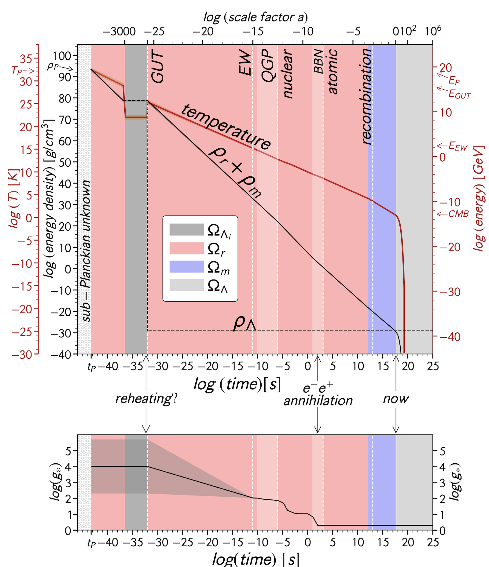
Fig. 2:  Top panel: Temperature and energy density of the universe as a function of time and of scale factor. Bottom panel: the relativistic degrees of freedom needed to compute the temperature and density for times less than a few minutes after the Big Bang. (Fig. 1 of Lineweaver & Patel 2023).

The top panel of Figure 2 shows the density and temperature of the universe as a function of time all the way back to the Planck time. To compute these, during the first few minutes of the history of the universe, one needs to know the number of relativistic degrees of freedom g* (bottom panel).  The standard model gives us good estimates of g* after the first ten billionth of a second: g*(t = 10^-10 s) = 106.75.  As we get closer to the Big Bang, for energies between 10² GeV and the Planck energy 10¹⁹ GeV, transitions in the underlying vacuum means g* depends on the model of high-energy physics.  For example, in heterotic superstring theory the number of different kinds of elementary particles is infinite. Or maybe g* → ∞ at the Hagedorn temperature? Unlike all subsequent billionths of a second, the first billionth of a second was special.

Unable to find specific predictions in this poorly understood regime, we made a linear extrapolation (surrounded by the grey cone to represent uncertainties).  Thus, the left side of the bottom panel of Fig. 2 is an explicit extrapolation into very speculative territory. Hopefully, the authors of high energy physics models will point us to the g* predictions of their models for t < 10^-10 s.  During inflation, in the absence of matter or radiation does g* → 1?

Astrophysicists will be interested in the small rectangle in Fig. 1 near the Sun and main sequence stars. Fig. 3 is a blow up of that region.

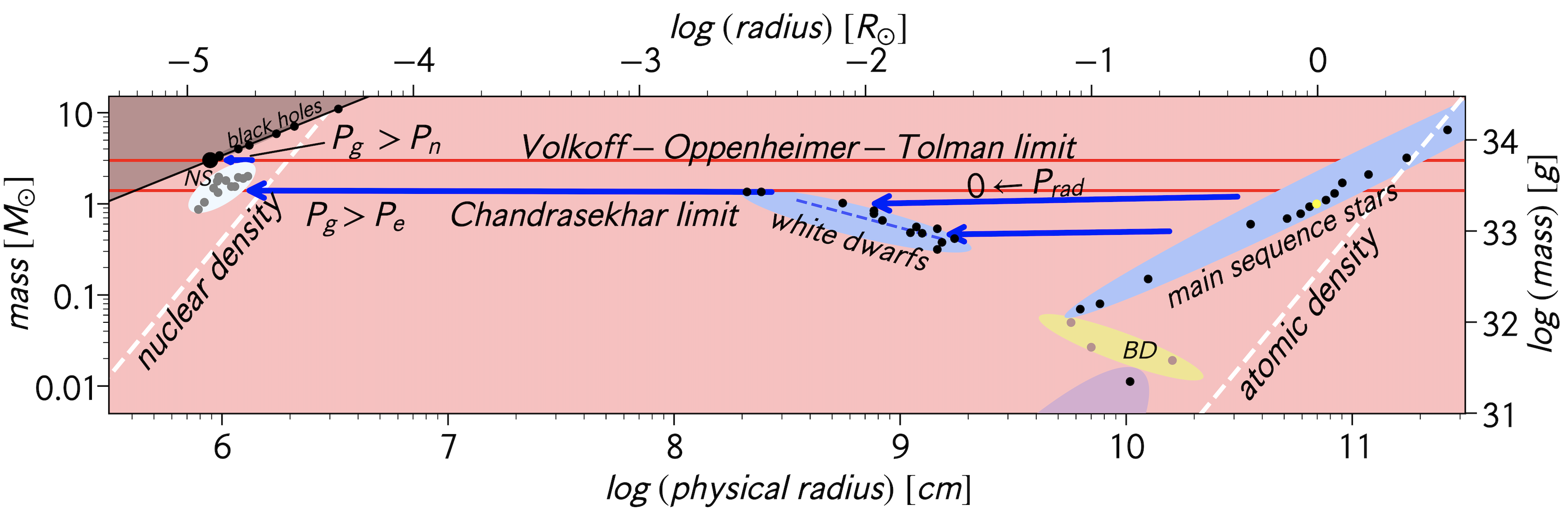
Fig. 3:  A zoomed-in version of the small black rectangle in Fig. 1 showing stellar evolution as a function of density. When main sequence stars (right) run out of fuel they collapse into white dwarfs held up by electron degeneracy pressure. When a white dwarf accretes material and its mass approaches the Chandrasekhar limit (~ 1.4 M_Sun) it becomes a neutron star (“NS”) held up by neutron degeneracy pressure. With further mass accretion, neutron stars become black holes, which lie on the black diagonal line in the upper left.  

For further details see Lineweaver, C.H. & Patel, V.M. (2023) “All objects and some questions”, American Journal of Physics 91, 10, 819-825./