The accurate measurement of physical constants is one of the main goals of research in subnuclear physics. On one side, it improves our ability to represent physical reality through our theoretical models, which opens the way to more stringent tests of our understanding of Nature; on the other, it allows us to test the internal consistency of the models themselves, which may lead to discoveries of new physical phenomena.

The measurement process sees experimenters engage in a fight with three enemies. The first enemy is statistical uncertainty. That is a source of imprecision connected with the intrinsic variability of our measurement process, which if repeated may return, under identical conditions, slightly different results. This is a quite general phenomenon, unrelated to the microphysics at the focus of our particle accelerator experiments; it rather has to do with the stochastic nature of basic ingredients of the observed phenomena, the measurement device, or both. For example, you might set out to measure the weight of a precious stone with a digital scale which reports weight in milligrams. If you perform the measurement several times, you will notice that the result changes every time, in an apparently random fashion. We have a powerful, if expensive, weapon to tame this annoying imprecision: averaging! If we take the average of several measurements, the variability of the result is reduced by the square root of the observations. This is, in a nutshell, why we need to collect large amounts of data: the more data we collect, the more precise our measurements become.

The second enemy, and the most dreaded one, is systematic uncertainty. Systematic uncertainty is tightly connected with the details of our measurement process: it is a bias resulting from imperfections of our instrument or of our measurement procedures. In the case of the weight of the precious stone mentioned above, a systematic uncertainty might result from a residual miscalibration of the scale, or a non-linearity of its response. Another cause of systematic uncertainty in the cited example could be the presence of grease or other dirt on the surface of the stone, liable to add to the stone’s reported weight.

While in the following we will discuss systematic uncertainties in more detail, for the sake of completeness we must recall that there is a third, often overlooked enemy to our ultimate precision. Whenever we set out to measure something, we implicitly assume that there is a “true” answer. But that is not always exactly the case. This third kind of error arises when the quantity we are estimating is not exactly well defined. For instance, if we want to know what our body weight is, we usually neglect to consider that our weight, as reported by even the most precise scale, depends not only on whether we had breakfast or not a moment ago: it also is affected by how much air there is in our lungs, how wet is our skin or our hair, etcetera. All of these are small imprecisions, of course; but they add to the overall complexity of the measurement process. Note that an ill-defined nature of the quantity under measurement is not alien to subnuclear physics; a striking example is the top quark. Top is the heaviest subnuclear particle we have so far discovered, and a lot of effort has gone, and is indeed still being invested, in the precise determination of its mass. But although the top quark is a well-defined object in quantum field theory, what we call its “mass” is not, because the particle can never be isolated completely from its environment – it is “strongly coupled” to other quarks and gluons by the action of the chromo-dynamical interaction, the strong force that binds quarks inside particles like the proton and the neutron.

While statistical uncertainty can be beaten down by collecting more data, and the error due to ill-defined nature of the quantity being measured is often small and ultimately something we have to live with, systematic uncertainties play a dominant role in determining the ultimate accuracy of our measurements, and their treatment is often what distinguishes a superb analysis from a mediocre one. A lot of effort consequently goes into trying to beat them down. Systematic uncertainties arising from controllable instrumental details are fought by designing better instruments, e.g. ones which produce more linear response, or which are easier to calibrate. But once our instruments are built, and data is taken, there is still a lot to do, as a number of systematic effects play a role in the analysis that produces the final results.

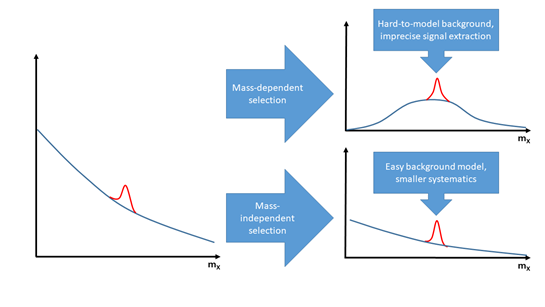
Let us focus on one of the most common analysis issues, by considering the measurement of the production rate at the LHC for a particle X which we may detect by sizing up the Gaussian-shape bump it produces in a reconstructed mass distribution (see Fig. 1, left). The typical challenge in estimating the number of events we can attribute to the decay of X is to beat down backgrounds (events which look like X decays but aren’t), such that the signal stands up more prominently in the resulting distribution. To do that, one selects signal-like events leveraging their observed properties. For each event, in fact, we measure a number of different variables in our detector: those “kinematic features” carry distinguishing power to tell signal events apart from backgrounds. Before machine learning became a thing, data selection was typically based on “straight cuts” on those features: if the signal is predominantly at high values of V, and background more frequent at low values of V, a requirement that data have V>V* (with the cut value V* chosen to optimize some suitable figure of merit) will usually do the job. Straight cuts increase the signal to background ratio, but they may be sub-optimal as they throw away significant information. Nowadays we employ for signal/background classification tasks tools such as neural networks or boosted decision trees: these algorithms outperform our cut-based selections by significant margins.

Whether we use cuts on event features or a powerful machine learning classifier, it usually happens that the resulting selection “reshapes” the background mass distribution (see Fig.1, top right). This should come as no surprise, since events at masses lower or higher than the mass of X can be safely discarded. The price to pay, however, is that it then becomes harder to precisely estimate the residual background in the selected data: the knowledge of how much background is present under the signal peak becomes a systematic uncertainty that may heavily affect our results. To reduce its impact, we may again rely on machine learning tools. A number of techniques have in fact been produced for that very specific task. The classifiers may be instructed to explicitly neglect the reconstructed mass of the target particle as a distinguishing feature; or they can be fed with signal generated at a bunch of different mass values, such that the algorithm will ignore mass in its classification task. Other successful ideas involve the explicit parametrization of the effect of the mass on the other variables, which helps remove the correlation between reconstructed mass and output of the classifier; or the use of weighted events in the training phase, such that the mass distribution becomes identical in signal and background events before the classification.

Figure 1: A reconstructed mass distribution for a particle X including background (blue curve) and signal events (red) allows the measurement of the signal rate more effectively if data selection is made independent on the value of the mass of the particle, as the background shape introduces fewer systematic uncertainty in the signal rate (bottom right).

In other cases, systematic uncertainties affect our results in less controllable ways. There are, for instance, many parameters describing the performance of our detectors which are not precisely known. Their values have an impact on the precision of the measurement because different assumptions on their unknown value produce shifts in our final estimates of the quantity we wish to measure. A wide set of different machine learning-based techniques has been developed to fight that resulting imprecision. If we still consider the classification task of separating an interesting signal from backgrounds, we may again imagine that a small variation δC of a calibration constant C in our detector will affect the measurement of one or more of the event features. This will make the classifier output different, and the fraction of signal passing a selection on its value will change by some corresponding amount, affecting the measurement in an undesirable way. How can we teach a neural network to become insensitive to the actual value of C? We can do it in many ways. We may penalize the network loss function – the value that the network is trying to minimize by adjusting its weights and biases during the learning process – if the output strongly depends on C. Or, we may pitch two neural networks one against the other, when the first tries to correctly classify signal events produced with simulations employing different values of C, while the other tries to learn the values of C from the features; the equilibrium point of such an “adversarial network” setup usually does the trick, if a stable solution can be found.

A very promising recent technique, called “INFERNO” leverages differentiable programming techniques recently made popular by tools such as TensorFlow and PyTorch (differentiable programming involves writing computer programs in such a way that every calculation can be subjected to automatic differentiation, enabling optimization of all its ingredients).  INFERNO solves the problem of systematic uncertainties more radically than other approaches, by injecting in the loss function of the classifier a direct, quantitative notion of the final accuracy of the measurement that results from the classification task once all systematic uncertainties are accounted for: by minimizing the loss, the network then learns the configuration which produces the best measurement. While the construction of the algorithm is indeed complex, the technique has been shown to perform excellently on synthetic problems, completely canceling the effect of multiple systematic uncertainties. The use of INFERNO and similar algorithms for the improvement of real analyses of LHC data is underway.

The above are examples of the benefits that machine learning methods can offer in data analysis. However, their potential is much higher. Indeed, it is my strong belief that the new frontier for experimental physics research is the exploitation of differentiable programming for a full optimization of experimental design, to include not just the accurate reconstruction of particle signals or the information-extraction procedures, but also the whole design of the detectors that produce the data themselves. When we design detectors we are trying to find the optimal working point in a space of design choices which is extremely high-dimensional, and the task is clearly super-human. A synergic optimization of detectors and data together, enabled by new computer science tools, will allow a realignment of our design to our scientific goals, offering huge dividends in terms of our knowledge gain per unit of investment spent. In a world plagued with global challenges (pandemics, overpopulation, climate change) which force us to direct our resources into applied science solutions, a more effective use of funding spent in fundamental science is what can ultimately save that essential human endeavor from a slow decline.