![]()
What is the likelihood function, and how is it used in particle physics?
In statistical data analysis, “likelihood” is a key concept that is closely related to, but crucially distinct from, the concept of “probability”, which is often a synonym in everyday English. In this article, I first lay some necessary foundations for defining likelihood, and then discuss some of its many uses in data analyses in particle physics including the measured value of a parameter, an interval expressing uncertainty, and hypothesis testing in various forms. A simple example also illustrates how likelihood is central to deep controversies in the philosophical foundations of statistical inference. More complex examples at the LHC include measurements of the properties of the Higgs boson.
Statistical models
Before delving into our discussion about the use of likelihood in high-energy physics, we should explore the concept of “statistical models”, which are the mathematical expressions that relate experimental observations to underlying theory or laws of physics. We let x stand for an arbitrarily large collection of observations such as tracks of particles in the ATLAS or CMS detectors. We let θ stand for a host of quantities (collectively called parameters) that include constants of nature in putative or speculative laws of physics, as well as all sorts of numbers that characterize the response of the detectors. For example, calibration parameters relate flashes of light in lead tungstate crystals to inferred amounts of energy deposited by high-momentum electrons.
Even if all values of θ are kept fixed, the observations x will exhibit intrinsic variability, either because of slight changes in conditions or more fundamentally because of the randomness in the laws of quantum mechanics that govern the interactions in particle physics and lead to statistical fluctuations. Therefore, statistical models, usually written in the form of p(x|θ) or p(x;θ), are not deterministic equations but rather probabilities or probability density functions (pdfs) for obtaining various x, given a set of parameters θ. Experiments provide observations of x, which are used by scientists for inferences about components of θ (for example the mass of the Higgs boson) or about the form of p itself (such as whether the Higgs boson or other not-yet-seen particles exist).
Defining “probability” is a long and difficult discussion beyond the scope of this article. Here I simply assume that our readers most likely learned the “frequentist” definition of probability (relative frequency in an ensemble) in their quantum mechanics courses or elsewhere, and use this definition in practice with Monte Carlo simulation or efficiency measurements.
The likelihood function
After obtaining the collection of observations x, we take the expression p(x|θ), evaluate it only for the specific x that was observed, and examine how it varies as θ is changed! This defines the likelihood function L(θ), often also denoted as L(x|θ) and sometimes L(θ|x):
L(θ) = p(x|θ), evaluated at the observed x, and considered to be a function of θ.
An additional overall arbitrary constant can be ignored. Importantly, while p(x|θ) expresses probabilities or pdfs for various x, the likelihood function L(θ) does not express probabilities or pdfs for θ. When Sir Ronald Fisher called it “likelihood” in the 1920s, his intent was to emphasize this important distinction. This definition of the likelihood function is general enough to include many special cases, for example where x includes properties of individual events (unbinned likelihood) as well where x includes the numbers of events in each bin of a histogram (binned likelihood).
Various uses of L(θ) are identified with at least three contrasting approaches to statistical inference, which in the following are referred to as “likelihoodist”, “Neyman-Pearson” (NP), and “Bayesian”. We illustrate them here with a statistical model p(x|θ) having a very simple mathematical form. But we must keep in mind that when we analyse real experimental data, L(θ) is only as valid as p(x|θ). Hence, great efforts go into specifying the mathematical form of p and obtaining values with uncertainties for the components of θ, which can number in the hundreds or even thousands. For this purpose, massive “calibration and alignment” efforts for detectors such as ATLAS and CMS are crucial, as are the many tests to ensure that the models capture the essential aspects of the experimental techniques. This need surely remains with the current trend toward using “machine learning” methods, within which computer algorithms develop numerical representations of p(x|θ) that can be difficult for humans to understand fully.
The Likelihoodist approach
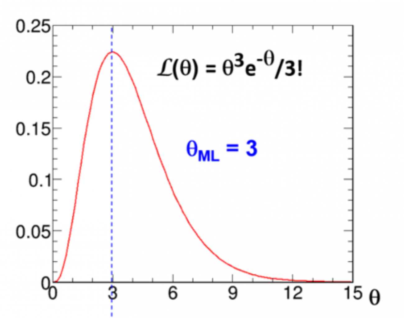
For illustration, we take as our statistical model the Poisson distribution that describes the probability of observing the integer x, which is the number of events that pass certain selection criteria. The value of x is sampled from the Poisson distribution with an unknown true mean θ:
p(x|θ) = θxe-θ/ x!.
Now suppose that the value that was actually observed is x=3. This means that the likelihood function is
L(θ) = θ3 e-θ / 6.
The likelihoodist approach (advocated by A.W.F. Edwards in his 1972 monograph, Likelihood) takes the likelihood function as the fundamental basis for the theory of inference. For example, the likelihood ratio L(θ0)/L(θ1) is an indicator of whether the observation x=3 favours θ=θ0 over θ=θ1. Edwards considered values of θ for which -2ln(L(θ)) are less than one unit from the minimum value of -2ln(L(θ)) to be well supported by the observation. Figure 1 contains graphs of L(θ) and -2ln(L(θ)). For values of θ at or near the maximum of L(θ) at θ=3, the observation x=3 had higher probability of occurring than for other values of θ.
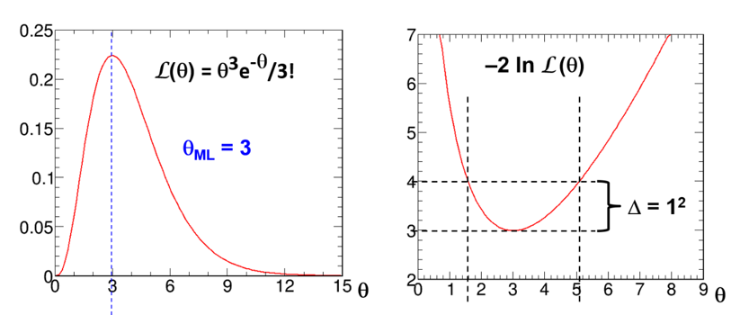
Figure 1. For the Poisson distribution, plots of the likelihood function L(θ) and -2ln(L(θ)) in the case that x=3 is observed. Since L(θ) is not a pdf in q, the area under L(θ) is meaningless. The maximum likelihood estimate is θML=3, and an approximate 68% CL confidence interval is [1.58, 5.08], obtained from Δ(-2ln(L(θ)))=1.
The Neyman-Pearson approach
Most modern data analysts find that the pure likelihoodist approach is too limiting, and that the likelihood (or ratio) needs to be supplemented in order to have a calibrated interpretation as strength of evidence. In the 1920s and 30s, Neyman and Pearson (NP) developed an approach to tests of hypotheses based on examining likelihood ratios evaluated not only at the observed value of x, but also at values of x that could have been observed but were not. This was generalized to constructing confidence intervals with associated confidence levels (CL) that are common today.
We introduce the NP theory with a somewhat artificial example. Let’s assume that we have one physics hypothesis (H0) that predicts exactly θ=θ0 and a second physics hypothesis (H1) that predicts exactly θ=θ1. Neyman and Pearson advocated choosing H0 if the likelihood ratio L(θ0)/L(θ1) is above some cut-off value. This cut-off value can be calculated from the experimenter’s desired maximum probability of choosing the second theory if the first theory is true (“Type I error probability”). The Neyman-Pearson lemma says that for any desired Type I error probability, choosing the correct theory based on a cutoff for this likelihood ratio will minimize the probability that the first theory is chosen when the second theory is true (“Type II error probability”).
A key aspect of this approach is that the calculations of the NP error probabilities involve evaluating p(x|θ) at all possible values of x (the “sample space”), not just at the observed value. In particle physics, the “number of σ” , or the equivalent p-value that is used as a measure of strength of evidence for an observation or discovery, is closely related, and shares this aspect.
In 1937, Neyman showed how to construct “confidence intervals” in θ (his phrase). The lower and upper endpoints [θL , θU] are functions of the observed x , as are Edwards’s intervals of support. The defining new feature was that one could choose a number called the “confidence level” (CL); 68% and 95% are common at the LHC. With x randomly sampled from the sample space according to the statistical model, the endpoints [θL, θU] are distributed such that the confidence intervals contain (“cover”) the unknown true value of θ in at least a fraction CL of the intervals, in the imagined limit of infinite repetitions. The phase “at least” is necessary when the observations are integers; for continuous observations, the coverage is exact in the simplest models.
In fact, the ensemble of confidence intervals need not be from the same statistical model. In principle, the set of measurements in the Particle Data Group’s Review of Particle Physics could serve as the ensemble, if all the statistical models were correctly described. There are, however, enough incompatible measurements in the listings to indicate that we have not achieved this ideal.
Meanwhile Fisher, who subscribed neither to the strict likelihoodist philosophy nor to NP testing, proved multiple theorems about the usefulness of using the “method of maximum likelihood (ML)” for obtaining the quoted measured value of θ (“point estimate”). He also studied the shape of the log-likelihood function (second derivative, etc.) as measures of uncertainty, as well as Fisher’s definition of “information” contained in the observation.
A common point of view nowadays is that intervals of support based on differences of -2ln(L(θ)), particularly as generalized by S.S. Wilks and others to the cases with models having many parameters θ, can be extremely useful as algorithms for constructing intervals and regions that approximately satisfy Neyman’s coverage criterion for confidence intervals. This approximation generally gets better as the data sample size increases. For example, ATLAS and CMS, separately and in combined results, relied heavily on log-likelihood differences for measurements of the mass and couplings of Higgs bosons to other particles [1,2], as illustrated below.
The Bayesian Approach
Finally, to introduce the Bayesian approach, we must consider a definition of probability other than the frequentist definition. An old view, which has attracted many adherents in the last half-century, is that probability is not something intrinsic to decaying particles (or rolling dice), but rather resides in an individual’s mind as “subjective degree of belief”. Nowadays the moniker “Bayesian” typically refers to this definition of probability. Whatever one thinks of this, it undoubtedly applies to more situations, particularly in a case with no relevant ensemble, such as “the probability that the first person on Mars returns to Earth alive”. One can define a continuous pdf for a presumed “constant of nature” such as the mass of the Higgs boson, from which one can calculates one’s belief that the mass is within some specified interval. (A frequentist pdf does not exist, or is useless.)
In the Bayesian framework, one has the “prior pdf” pprior(θ) that specifies relative belief in values of θ before the observation x is incorporated into belief. Afterwards one has the “posterior pdf” pposterior(θ|x), given the observed x. The celebrated Bayes's Theorem, which applies both to frequentist probabilities (when they exist) and to Bayesian probabilities, implies the proportionality,
pposterior(θ) ∝ L(θ) x pprior(θ).
The likelihood function (which is not a pdf in θ), relates the before-and-after beliefs about θ in this simple way. The posterior pdf can then be used for a variety of purposes, including “credible intervals” that correspond to specified levels of belief.
Among the controversies with this approach, including whether Bayesian probability is a useful concept for scientific communication, are those involving the choice of the prior pdf. Choices representing an individual’s degree of belief may be objectionable to those with other beliefs. A completely different way to obtain prior pdfs for θ is to use formal mathematical rules applied to the functional form of the model p(x|θ) [3]. These so-called “objective priors” depend on the measurement apparatus and protocol!
As an example, if a measurement apparatus has a Gaussian resolution function for the mass, the usual formal rules dictate a prior pdf uniform in mass. But if a different measurement apparatus has a Gaussian resolution function for the mass-squared, then a prior pdf uniform in mass-squared is dictated. By the rules of probability, the latter implies a prior pdf for mass that is not uniform in mass. As startling as that may seem, the formal rules can bring some perceived advantages, and even help forge a connection to Neyman’s frequentist notion of coverage [3].
In particle physics, with its strong tradition of frequentist coverage, prior pdfs are often chosen to provide intervals (in particular upper limits for Poisson means) with good frequentist coverage [4]. In such cases, our use of Bayesian computational machinery for interval estimation is not so much a change in paradigm as it is a technical device for frequentist inference.
The Likelihood Principle
This simple Poisson model highlights a fundamental difference between, on the one hand, NP testing and related concepts common in particle physics, and on the other hand, the likelihoodist and Bayesian approaches. After data are obtained, the latter adhere to the “Likelihood Principle”, which asserts that the model p(x|θ) should be evaluated only at the observed x. In contrast, the usual confidence intervals and measures of “statistical significance” reported in particle physics (3σ, 5σ, etc.) include concepts such as the probability of obtaining data as extreme or more extreme than that observed. This deep philosophical issue, which also leads to differences in how one treats the criteria by which one stops taking data, remains unresolved [4].
In the limit of large samples of data, the three approaches for measurements of quantities such as the Higgs boson mass typically yield similar numerical values, all having good coverage in the sense of Neyman, so that any tension dissipates. In fact, both the likelihoodist and Bayesian approaches can provide convenient recipes for obtaining approximate confidence intervals. However, the likelihoodist and Bayesian conclusions when testing for a discovery can be quite different from the usual “number of σ” in common use in particle physics, even (especially!) with large data sets [5].
Beyond the simple Poisson example
The discussion becomes substantially richer when there are two observations of x, and/or two components of θ, still within the context of one statistical model [4]. Another generalization is when a second experiment has a different statistical model that contains the same set of parameters θ and an independent set of observations y. Then the likelihood function for the combined set of observations x and y is simply the product of the likelihood functions for each experiment. In the case of ATLAS and CMS, each experiment has its own statistical model, reflecting differences in the detectors, while having in common underlying laws of physics and constants of nature. A meta-model for the combination of the two experiments requires understanding which parameters in each statistical model are unique, and which correspond to parameters in the other experiment’s statistical model. For measurements of the Higgs boson mass and properties, the collaborations invested significant resources in preforming such combinations [1,2].
Frequently, one is particularly interested in one or two components of the set of parameters θ, regardless of what the true values are of all the other components of θ. Each of the three approaches that we presented (likelihoodist, NP, Bayesian) has its associated method(s) for “eliminating” these other “nuisance parameters” [4]. No method is entirely satisfactory, and sometimes a pragmatic synthesis is preferred. The interested reader can pursue the topics of “integrated likelihood” and “profile likelihood”. By convention, the latter is commonly used by both ATLAS and CMS, including in the figures shown here.
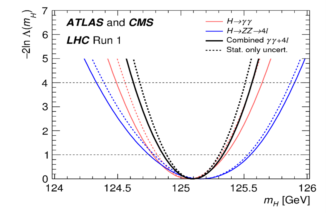
Figure 2. Solid black curve: Measurement of the mass mH of the Higgs boson using the likelihood function L(mH) from the first combination of ATLAS and CMS data [1]. The ML estimate is m̂H= 125.09GeV. The curves are -2ln(Λ(mH)), where Λ = L(mH)/L(m̂H), with nuisance parameters treated by profile likelihood [1] and suppressed in the notation here. Approximate 68% CL and 95% CL confidence intervals are indicated by the increases of 1 and 4 units. The other curves indicated in the legend are described in Ref. [1].
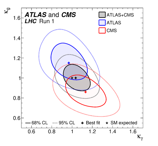
Figure 3. For the two parameters of interest (kγ,kg) described in the text, the curves in the plane are contours of -2ln(L(kγ,kg)) from the combination of ATLAS and CMS data, and for each experiment separately [2]. As described in Ref. [2], the likelihood ratios used to calculate each contour correspond to approximate 68% CL and 95% CL confidence regions in the two-parameter plane. The crosses labeled “Best fit” indicate the ML estimates of the two parameters.
Figures 2 and 3 are example plots for ATLAS-CMS combined measurements from the first LHC run. In Fig. 2 [1], the parameter of interest was the Higgs boson mass mH. Figure 3 [2] is part of a study of great interest to see if the Standard Model (SM) correctly predicts the coupling of the Higgs bosons to two photons, as well as that to two gluons. Two parameters of interest, kγ and kg, were defined to be unity in the SM, and possible departures were measured. With this initial level of precision, no significant departure was observed.
In conclusion, we see that while the likelihood function is not a pdf in the parameter(s) of interest, it has multiple uses in the various approaches to statistical inference, all of which depend on an adequate statistical model. There are many pointers to the likelihood literature in the references below.
References
[1] ATLAS and CMS collaborations, “Combined Measurement of the Higgs Boson Mass in pp Collisions at √s = 7 and 8 TeV with the ATLAS and CMS Experiments,” Phys. Rev. Lett. 114 (2015) 191803. https://arxiv.org/abs/1503.07589 .
[2] ATLAS and CMS collaborations, “Measurements of the Higgs boson production and decay rates and constraints on its couplings from a combined ATLAS and CMS analysis of the LHC pp collision data at √s = 7 and 8 TeV,” JHEP 08 (2016) 045. https://arxiv.org/abs/1606.02266 .
[3] R. E. Kass and L. Wasserman, “The selection of prior distributions by formal rules”, J. Amer. Stat. Assoc. 91 (1996) 1343. http://www.jstor.org/stable/2291752 . doi:10.2307/2291752.
[4] R. D. Cousins, “Lectures on Statistics in Theory: Prelude to Statistics in Practice” https://arxiv.org/abs/1807.05996 (2018)
[5] R. D. Cousins, “The Jeffreys–Lindley paradox and discovery criteria in high energy physics”, Synthese 194 (2017) 395, https://arxiv.org/abs/1310.3791 . doi:10.1007/s11229-014-0525-z, 10.1007/s11229-015-0687-3.